Cross-Talk Compensation Using Matrix Methods

Force sensors are designed to measure forces and torques along defined axes, typically labeled X, Y and Z. These force sensors can have from one to six measurement channels; three force channels (Fx, Fy and Fz) and three torque or moment channels (Mx, My and Mz). In theory, a load along any one of those measurement axes will not produce an output on any of the other measurement channels. Unfortunately, this is seldom the case in the real world. For most force sensors, this un-desired output, or cross talk, will be between 1 and 5%. While 1% – 5% cross talk may not sound like much, if each channel has 1% – 5% cross talk due to each of the remaining five loads, then the total cross talk could be as high as 5% – 25%.

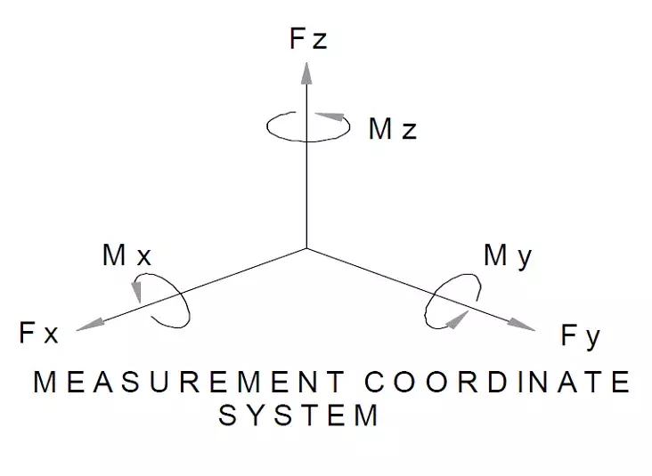
There are basically two methods used to reduce this potential source of measurement error. With the first method, the load-cell is ‘tuned’, either mechanically or electrically to reduce the channels output due to off-axis or extraneous loads. While effective, this method is time consuming and is not practical if more than two extraneous loads need to be compensated for. The other method of cross-talk compensation involves mathematically manipulating the load-cells output data to correct the cross-talk outputs. It is effective for any number of extraneous loads, and can be characterized as mathematical cross-talk compensation by the application of “cross coupling coefficients”, or the inverse matrix method. This is the method that will be discussed here.

When a load is applied to a force sensor, the measurement channel that lines up with that load will respond. However, as described earlier, other measurement channels that are not in line with that applied load will also respond to that load. That’s the bad news. The good news is that that response is repeatable for any given load or combination of loads. This means that by carefully applying these extraneous loads during the calibration process, and recording each channels output response to those loads, an output profile of the sensor can be created. From here, a series of simultaneous equations can be created to describe the cross-talk performance of the force sensor. By solving this series of equations using any set of simultaneous data from all the channels of the sensor, the true loading condition that produced that unique set of data can be determined. The drawback to this method is that a sensor channel is required for each extraneous load that is present during loading. This usually isn’t a problem, since in most instances, a measurement channel is present to monitor all the significant loads present in the application.

In application, a six-axis sensor, with three force channels and three torque channels, will be calibrated by applying a known load in line with one of those measurement axis, and recording the output from the corresponding channel. This gives rise to the first transfer function for the sensor. That is, the channel output, O, is equal to the sensitivity (mV/V per unit load), K, times the applied load, F, or:

OFx = K1 ·Fx

At the same time, the output from the other five channels will be recorded as cross talk outputs. Now the transfer functions for the sensor begin to take shape.

OFx = K1 ·Fx

OFy = K7 ·Fx

OFz = K13 ·Fx

OMx = K19 ·Fx

OMy = K25 ·Fx

OMz = K31 ·Fx

From this set of equations, the transfer functions (K1, K7, etc), can be determined for each axis by dividing the sensors output by the applied load. This same procedure will be used to calibrate the remaining five axes of the sensor, providing the remaining transfer functions. Using the theory of superposition, they can be combined to yield the output equations that fully describe the output of the sensor to all the applied

loads.

OFx = K1·Fx + K2·Fy + K3·Fz + K4·Mx + K5·My + K6·Mz

OFy = K7·Fx + K8·Fy + K9·Fz + K10·Mx + K11·My + K12·Mz

OFz = K13·Fx + K14·Fy + K15·Fz + K16·Mx + K17·My + K18·Mz

OMx = K19·Fx + K20·Fy + K21·Fz + K22·Mx + K23·My + K24·Mz

OMy = K25·Fx + K26·Fy + K27·Fz + K28·Mx + K29·My + K30·Mz

OMz = K31·Fx + K32·Fy + K33·Fz + K34·Mx + K35·My + K36·Mz

These equations describe the output of the sensor in terms of the applied loads. However, in application, the loads are the unknowns, and the outputs are the known measured quantities. With these six equations and their six unknowns (the loads Fx-z and Mx-z), it will be possible to solve for the unknown loads.

Inverse Matrix Method

The series of equations described above can be solved by using what is called the inverse matrix method. A brief overview of the theory behind this technique is given in Appendix A, ‘Inverse Matrix Theory’. In essence, it is a technique that ‘inverts’ the equations so that instead of having the output as a function of the loads as described above, the loads are now functions of the outputs.

Finding the inverse matrix used to correct or compensate a sensors output due to cross talk errors, involves gathering calibration data on the sensors response to extraneous loads, and using it to construct a matrix that can be used to find the sensors true loading condition. A multi-axis sensor that has undergone a thorough calibration, will already have such a cross talk matrix supplied with the calibration data. More information on the steps involved in creating this matrix is presented in Appendix B, ‘Finding the Inverse Matrix’.

This may all seem confusing, but it is a very simple way to handle a very complex problem. For example, we have a sensor that is ‘less than perfect’. We do however have the cross-talk matrix that was supplied with the sensor, as listed below.

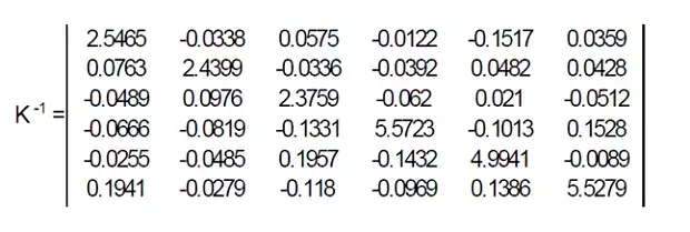
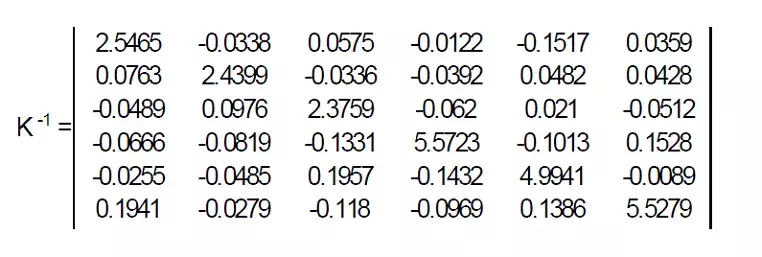
With this inverse matrix the loads that produced any set of simultaneous data from the sensor can be calculated. We start with the inverse matrix, K-1, and the equation: X = K^-1xO

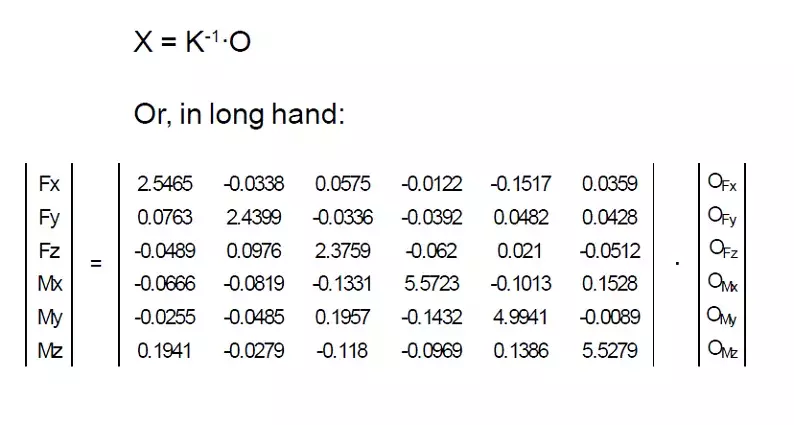
At a particular point in time, we obtain the following readings from our sensor:

OFx = -1.6510 mV/V OMx = 1.0054 mV/V

OFy = 0.6151 mV/V OMy = 0.8402 mV/V

OFz = 0.2501 mV/V OMz = 0.0067 mV/V

To find the Fx load that must have been present to create those six outputs, we multiply the elements of the first row of the inverse matrix by the individual outputs that were recorded, and sum them:

Fx = (2.5465 * -1.6510) + (-0.0338 * 0.6151) + … + (0.0359 * 0.0067) = -4.35 lb

Similarly, the remaining five loads can be calculated by carrying out the same operations on the remaining five rows of the inverse matrix. Doing so yields the following loading conditions:

Fx = -4.35 lb Mx = 5.54 in lb

Fy = 1.37 lb My = 4.11 in lb

Fz = 0.69 lb Mz = -0.31 in lb

In actual use, these calculations can be set up to be done in real time by the data acquisition or control system, or can be done by post processing the data after the test is complete by using a spread sheet program. This technique will typically reduce the cross talk to less than 0.5% of the full-scale capacities of the sensor.

APPENDIX B

FINDING THE INVERSE MATRIX

In order to find the inverse matrix that will be used to compensate for cross talks due to extraneous loads, the sensors response to those individual extraneous loads must be determined. For example, let’s say we have a six-axis sensor with 5 lb capacities for the force channels, and 10 in.lb capacities for the moment channels. It has been calibrated by applying those loads, one at a time, and monitoring the individual sensor channels. The following data has been collected:

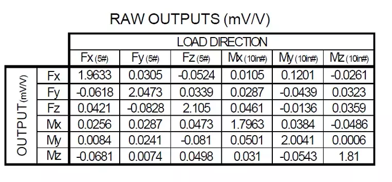
By dividing the channel output due to an extraneous load, by the full-scale output for that same channel, the sensors cross talk performance can be seen.

CROSS TALK PERFORMANCE (% Full Scale Output)

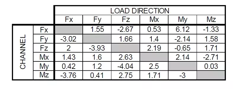
Here, the minimum cross talk is only 0.03% of the full-scale load when an Mz load is applied to the My channel. If all the values were this good, no correction would be necessary. However, the maximum is over 6%, and the average cross talk for this sensor is around 2%. Computed cross talk compensation will definitely improve the accuracy of the data obtained from this sensor. The data matrix, referred to as ‘K’ in Appendix A, is constructed by taking the cross-talk data and dividing it by the applied load, to get the transfer function for that load / channel combination.

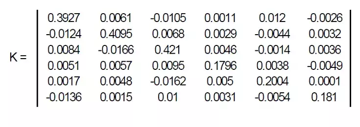
Using a computer program such as Excel, the inverse of this matrix is easily calculated using built in functions, and is shown below:

An interesting thing about matrices and their inverses is that when they are multiplied together, either as K·K-1 or as K-1·K, the result is what is called an identity matrix, that is, a matrix with 1’s along its diagonal, and 0’s in all the other locations, like this

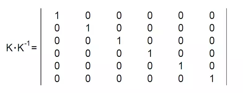
Performing this operation is often done to verify the inverse matrix was correctly derived.